Noise is everywhere—cosmic rays flip bits in RAM, replication errors corrupt DNA, servers crash, ledgers get unbalanced. The solutions have different names depending on who's solving the problem: fault tolerance, DNA mismatch repair, replication, double-entry bookkeeping. But the underlying principle is the same: encode information with more structure than strictly necessary, so we can detect and correct errors when they violate that structure.
In this post, I'll show how this principle works in quantum computing through quantum error correcting codes (QECCs). Unlike classical bits, quantum information is extraordinarily fragile. It can't be copied, and measuring it destroys it, yet we still need to protect it from noise. I'll start with classical error correcting codes, then show how quantum mechanics forces a fundamentally different approach.
Error Correcting Codes
You have $k$ bits of information that must pass through a noisy channel, like a transmission line with interference, a disk that might degrade, or stick of RAM vulnerable to cosmic rays. Some bits will randomly flip. How do you prevent the information from getting corrupted?
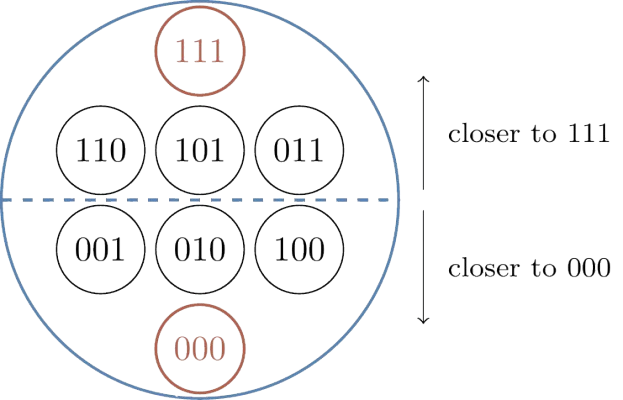
The simplest solution is simply to add redundancy by repeating each bit $n$ times. A 0 becomes $\underbrace{00\ldots0}_n$, and 1 becomes $\underbrace{11\ldots1}_n$. When noise flips some bits, we recover the original by majority voting: count the 0s and 1s, decode to whichever is more common. If we start with 000 and one bit flips to give 010, two 0s outvote one 1, correctly recovering 0. This works as long as fewer than half the bits flip—if noise corrupts the majority, the vote fails.
The 3-bit repetition code can correct 1 error but not 2. If two bits flip (say 000 → 110), the corrupted string has two 1s and one 0, so majority voting incorrectly decodes to 1. To correct more errors, you need more repetitions: a 5-bit code can correct 2 errors, a 7-bit code can correct 3, and so on. In general, an $n$-bit repetition code can correct up to $\lfloor(n-1)/2\rfloor$ errors. More protection requires more physical bits—this is the fundamental tradeoff. Repetition works but is wasteful. Can we do better?
Parity Checks
How to improve on repetition? We still add extra bits (redundancy is unavoidable), but instead of copying data directly, we add bits that encode relationships between the data bits. A parity check computes whether a set of bits has even or odd parity. For example, take data bits 101. Their parity is $(1 + 0 + 1) \bmod 2 = 0$ (even). Append this as a parity bit to get 1010. If an error flips the second bit to give 1110, recomputing the parity yields $(1 + 1 + 1) \bmod 2 = 1$, which doesn't match the stored parity (0). The mismatch tells us an error occurred—but not which bit flipped.
To locate errors, use multiple overlapping parity checks. The Hamming(7,4) code (developed by Richard Hamming in 1950) takes 4 data bits d₁, d₂, d₃, d₄ and adds 3 parity bits p₁, p₂, p₃. Each parity bit checks a different subset of the data bits. The structure is captured by three overlapping circles, where each circle represents a parity check, and each data bit sits in a region covered by a specific subset of checks.
Each parity bit checks all positions within its circle. For example, p₁ (blue) checks d₁, d₃, and d₄; p₂ (green) checks d₁, d₂, and d₄; p₃ (red) checks d₂, d₃, and d₄. When an error flips d₄ (in the center where all three circles overlap), all three parity checks fail. But if an error flips d₁ (blue-green overlap only), then p₁ and p₂ fail while p₃ passes. Each of the seven positions produces a unique pattern of parity check failures.
This pattern—which parity checks passed and which failed—is called the syndrome. Since there are 3 parity checks, you get $2^3 = 8$ possible syndromes—enough to uniquely identify which of the 7 bits flipped, or that no error occurred. Importantly,
For classical codes this seems like a technical detail, but for quantum codes it's essential: measuring quantum data directly would destroy the superposition we're protecting, so we can only measure syndromes.
Hamming(7,4) can correct 1 error but uses only 7 bits to protect 4 data bits—much more efficient than repetition's 3 bits to protect 1. More sophisticated codes achieve even better tradeoffs. The best classical codes are asymptotically good: they can correct a number of errors that grows proportionally with the code size, while keeping a constant fraction of bits as data (unlike repetition codes, where the data fraction vanishes).
But there's a catch: while encoding is straightforward (compute the parity checks and append them), decoding—recovering the original data from corrupted bits—becomes computationally hard. The decoder's job is to look at the received bits, figure out which errors likely occurred, and correct them. For repetition codes, this is trivial: take a majority vote. For the Hamming code, check which syndrome you got and flip the corresponding bit. But for asymptotically good codes, the problem becomes exponentially harder—there are exponentially many possible error patterns, and finding the most likely one is NP-hard in general. This computational challenge becomes even more severe in quantum codes, where decoding must happen in microseconds as the quantum computer runs.
Quantum Error Correction
The same redundancy principle survives in quantum systems, but the constraints are fundamentally different. The no-cloning theorem prohibits making copies of unknown quantum states, ruling out simple repetition. Measuring a quantum state destroys its superposition, so we can't just "read" qubits to check for errors. Yet despite these constraints, quantum error correction is possible—we just need to rethink what we can measure.
A classical bit is either 0 or 1. A qubit exists in a superposition: $$|\psi\rangle = \alpha|0\rangle + \beta|1\rangle \equiv \begin{bmatrix} \alpha \\ \beta \end{bmatrix}$$ where $\alpha, \beta$ are complex numbers satisfying $|\alpha|^2 + |\beta|^2 = 1$. The amplitudes $|\alpha|^2$ and $|\beta|^2$ determine the probabilities of measuring 0 or 1, while their complex arguments encode a phase—a relative angle that affects how qubits interfere when they interact.
This isn't just classical uncertainty. If you have a probabilistic classical bit that's heads with 50% probability and tails with 50%, it's secretly one or the other—you just don't know which. A qubit in superposition $\frac{1}{\sqrt{2}}(|0\rangle + |1\rangle)$ is genuinely both at once. When quantum operations combine these amplitudes, they interfere—they can add constructively (reinforcing each other) or destructively (canceling out), depending on their relative phases. This is what makes quantum computing powerful: algorithms manipulate these amplitudes to amplify correct answers and suppress wrong ones. It's also what makes errors so destructive—errors corrupt the delicate phase relationships, turning constructive interference into destructive interference.
Errors can corrupt quantum information in two ways. A bit flip swaps $|0\rangle \leftrightarrow |1\rangle$ (equivalently, $\alpha \leftrightarrow \beta$). A phase flip changes the sign of one component, say $|1\rangle \to -|1\rangle$ (equivalently, $\beta \to -\beta$). These correspond to Pauli operators $X$ and $Z$; a combined error $Y$ does both. In matrix form $X=\begin{bmatrix}0 & 1\\ 1 & 0\end{bmatrix}$ swaps the entries of $\begin{bmatrix}\alpha\\\beta\end{bmatrix}$, while $Z=\begin{bmatrix}1 & 0\\ 0 & -1\end{bmatrix}$ keeps the top entry and flips the sign of the bottom. Phase errors are invisible if you measure the qubit directly—measurement only reveals $|\alpha|^2$ and $|\beta|^2$, not the phase—but they corrupt the relative angle between computational basis states, which matters for quantum algorithms. Classical error correction only needs to worry about bit flips; quantum error correction must protect against both bit flips and phase flips simultaneously.
The key constraint: measuring a qubit collapses it to a definite 0 or 1, destroying the superposition. This makes quantum error correction fundamentally different from classical. We can't just "read" qubits to check for errors. Instead, we must measure relationships between qubits—parity checks that reveal whether an error occurred without revealing the state itself.
Here's what measuring a relationship looks like. Take two qubits and measure the operator $ZZ$—this asks "do these qubits have the same parity?" The measurement returns $+1$ if they're both $|0\rangle$ or both $|1\rangle$, and $-1$ if they differ. Crucially, this tells you the relationship (same or different) without telling you the individual values.
In matrix form, $ZZ = Z \otimes Z = \mathrm{diag}(1,-1,-1,1)$, so $|00\rangle$ and $|11\rangle$ are $+1$ eigenvectors and $|01\rangle, |10\rangle$ are $-1$ eigenvectors. If the qubits are in the entangled state $\frac{1}{\sqrt{2}}(|00\rangle + |11\rangle)$, measuring $ZZ$ returns $+1$ with certainty (since both terms have matching qubits), yet the individual qubits remain in superposition. If an error flips one qubit to give $\frac{1}{\sqrt{2}}(|01\rangle + |10\rangle)$, the $ZZ$ measurement returns $-1$ (mismatched parity), signaling an error without revealing which qubit flipped or what the original state was.
This is the key principle: we continuously measure these multi-qubit parity checks to detect when errors violate the expected relationships, then use the pattern of violations—the syndrome—to infer and correct the error. Like an accountant verifying that debits equal credits without knowing the actual dollar amounts involved, we can check if the books balance without learning what the numbers are.
But what about phase errors? Here's where quantum measurement gets subtle: you can measure a qubit in different bases, and each basis reveals different information. Measuring $Z$ distinguishes $|0\rangle$ from $|1\rangle$ (the computational basis). Measuring $X$ distinguishes $|+\rangle = \frac{1}{\sqrt{2}}(|0\rangle+|1\rangle)$ from $|-\rangle = \frac{1}{\sqrt{2}}(|0\rangle-|1\rangle)$ (the superposition basis); these are the $\pm 1$ eigenvectors of $X$. If we measure $|+\rangle$ in the $X$ basis, we definitely get the $+1$ outcome. If we measure $|-\rangle$, we get $-1$. But both give us 0 or 1 with 50/50 probability in the $Z$ basis.
Notice that a phase error flips the relative sign: $|0\rangle+|1\rangle \to |0\rangle-|1\rangle$, which means $|+\rangle \to |-\rangle$. In the $X$ basis, a phase error is a bit flip. So to detect phase errors, we just measure $XX$ stabilizers instead of $ZZ$ stabilizers.
This reveals why phase errors matter and why $Z$ measurements can't detect them. If you measure a qubit in the $Z$ basis, the states $|+\rangle$ and $|-\rangle$ both give you 0 or 1 with 50/50 probability—they're indistinguishable. The phase error is invisible. But if you measure in the $X$ basis, $|+\rangle$ and $|-\rangle$ are distinguishable, and the phase error shows up as a definite flip. Conversely, a bit flip error ($|0\rangle \to |1\rangle$) is obvious to $Z$ measurements but invisible to $X$ measurements, since both $|0\rangle$ and $|1\rangle$ are equal superpositions of $|+\rangle$ and $|-\rangle$.
This duality is why quantum error correction needs two types of stabilizers. $Z$-type stabilizers like $ZZ$ or $ZZZZ$ detect bit flip errors. $X$-type stabilizers like $XX$ or $XXXX$ detect phase errors. Each type of check catches what the other is blind to.
Algebraically, these are tensor products of Pauli matrices with eigenvalues $\pm 1$; measuring them projects the state onto the corresponding eigenspace, revealing only whether the expected parity held. A complete quantum error correcting code must have both types of stabilizers, arranged so their measurements don't interfere with each other—this constraint is what determines which codes are possible.
The Surface Code
The most studied quantum error correcting code is the surface code. It arranges data qubits on a 2D grid, with $X$-type and $Z$-type stabilizers living on alternating faces of the lattice. You can think of each stabilizer as a parity check on the four qubits around a square: it reports whether an even or odd number of them flipped. Each stabilizer involves only the four neighboring data qubits, making measurements local and relatively easy to implement in hardware.
A distance-$d$ surface code uses a $d \times d$ grid, encoding one logical qubit into roughly $d^2$ physical qubits. A logical error corresponds to an error chain that stretches across the grid; distance $d$ is the length of the shortest such chain. The distance determines fault tolerance: a distance-$d$ code can correct up to $\lfloor(d-1)/2\rfloor$ data-qubit errors. Larger grids mean more protection, but also more physical qubits.
In practice, we don't just measure stabilizers once—we measure them repeatedly over time, because the measurements themselves can be faulty. Comparing outcomes across rounds lets us tell a measurement blip from a persistent data error. This gives the syndrome a spacetime structure: two spatial dimensions (the grid) plus one temporal dimension (the measurement rounds). An error that persists across multiple rounds looks different from a measurement error that appears and disappears. The decoder must interpret this full 3D syndrome to figure out what happened.
Just as the Hamming(7,4) code encodes 4 data bits into 7 physical bits, a distance-$d$ surface code encodes one logical qubit into roughly $d^2$ physical qubits. The surface code protects this logical qubit from errors: if too few physical qubits experience errors, the decoder can figure out what went wrong from the syndrome and correct it, preserving the logical quantum information. But if too many errors occur—specifically, if an error chain stretches all the way across the lattice—the code fails. This is a logical error, and it means the encoded quantum information has been irreparably corrupted.
Recall that in the Hamming code, each syndrome uniquely identifies which bit flipped. Quantum codes are different: many different physical error patterns can produce the same syndrome. This is called degeneracy, and it's unavoidable—it's a consequence of measuring only relationships, not the qubits themselves. But degeneracy isn't a problem. The decoder's job isn't to identify exactly which errors occurred; it's to find any correction that prevents a logical error. If errors $E_1$ and $E_2$ produce the same syndrome and neither causes a logical error, the decoder can pick either one. What matters is the syndrome pattern: does it indicate that an error chain crossed the lattice? If not, any correction consistent with the syndrome will work.
This gives us a way to measure performance. If the physical error rate (the probability that any given qubit experiences an error) is $p$, the logical error rate $p_L$ is the probability that the code fails—that a logical error occurs despite the decoder's best efforts. For a good code and decoder, there's a critical threshold physical error rate $p_\text{th}$. Below threshold, increasing the code distance $d$ exponentially suppresses logical errors: $p_L \sim \left(\frac{p}{p_\text{th}}\right)^{(d+1)/2}$. Above threshold, larger codes don't help. For surface codes with near-optimal decoders, the threshold is around 1%—if physical qubits are better than this, scaling up the code makes logical qubits arbitrarily reliable.
Beyond Surface Codes
The surface code is elegant and well-understood, but it has a serious drawback: terrible efficiency. To encode one logical qubit with distance $d$, you need $O(d^2)$ physical qubits. A distance-10 code needs ~100 physical qubits for a single logical qubit. For large-scale quantum computing, this overhead is prohibitively high.
Quantum LDPC codes solve this problem. Just as classical LDPC codes achieve better rate-distance tradeoffs than repetition codes, quantum LDPC codes can encode many logical qubits with far less overhead than surface codes. They're more complex: stabilizers can involve qubits that aren't spatially adjacent, and the structure is no longer a simple 2D grid.
Bivariate bicycle (BB) codes are a recent example. These are defined on a torus—imagine taking a rectangular grid and gluing the top edge to the bottom, and the left edge to the right, so that moving off one side wraps around to the other. The code's stabilizers are specified by polynomial equations over this toroidal geometry.
The efficiency gains are dramatic. The $[[144, 12, 12]]$ BB code encodes 12 logical qubits into 144 physical qubits with distance 12. Compare that to surface codes: achieving distance 12 would require roughly 144 physical qubits for one logical qubit. BB codes give us 12× better encoding rate at the same distance. For building large quantum computers, this difference is enormous.
| Surface Code | BB Code $[[144,12,12]]$ | |
|---|---|---|
| Physical qubits | ~144 | 144 |
| Logical qubits | 1 | 12 |
| Distance | ~12 | 12 |
| Rate ($k/n$) | ~0.7% | 8.3% |
| Geometry | 2D planar grid | Torus |
Decoding
We now have codes that can protect quantum information with excellent efficiency. The problem is that codes are useless without a decoder: the algorithm that looks at the syndrome (which stabilizers were violated, across all measurement rounds) and decides what correction to apply.
The decoder must satisfy two competing demands. It must be accurate: correctly identifying errors even when they're rare, because a single undetected logical error can ruin an entire computation. And it must be fast: syndromes arrive continuously as the quantum computer runs, and the decoder must keep up. For superconducting qubits, this means processing each round in about a microsecond. For trapped ions or neutral atoms, the budget is closer to a millisecond—more relaxed, but still demanding.
For surface codes, elegant algorithms based on graph theory work remarkably well. But for quantum LDPC codes like BB codes, decoding is much harder. The standard approaches either fail outright or are too slow for real-time use. This is where machine learning enters the picture—but that's a story for Part 2.